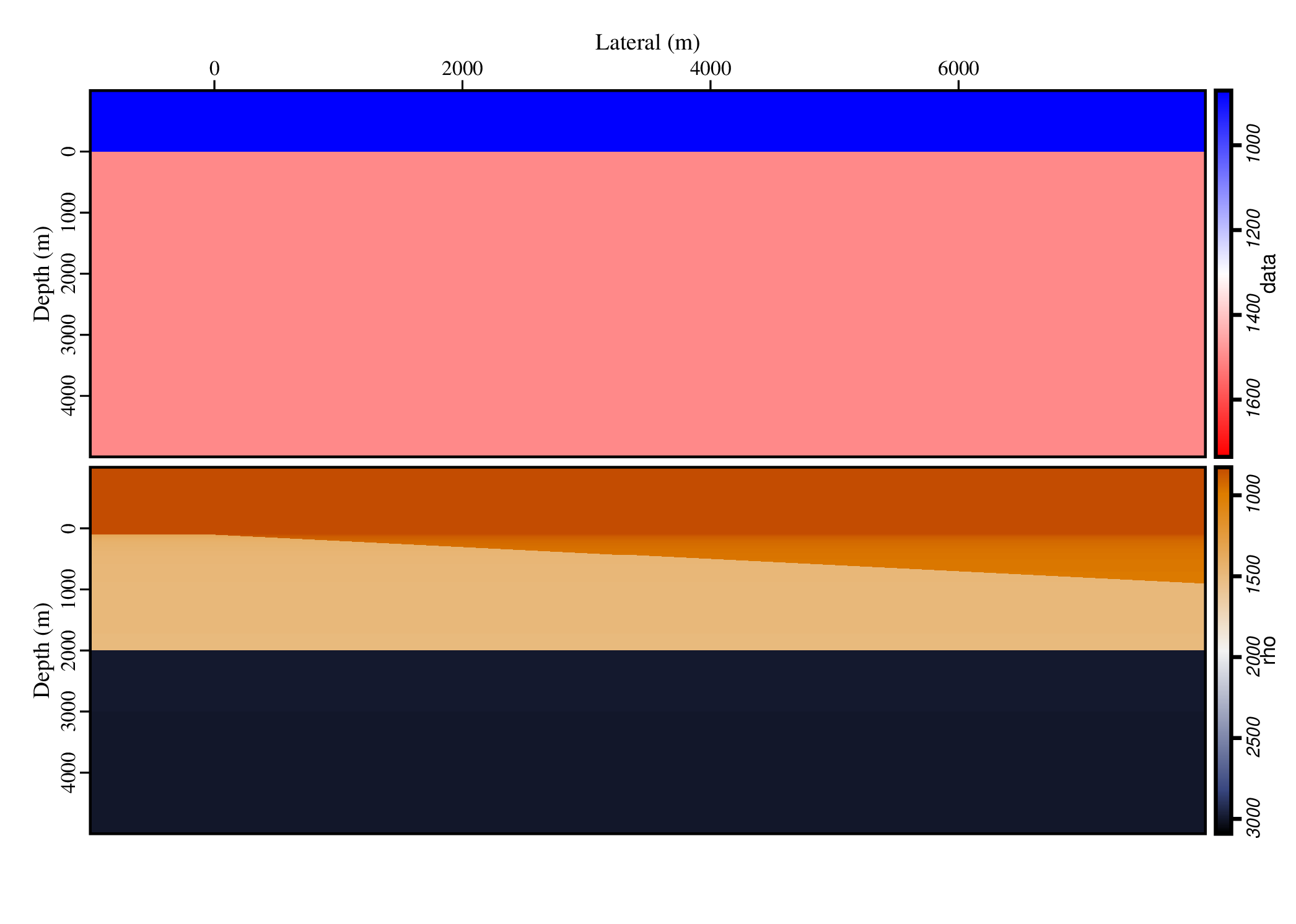
- We create a velocity model and a density model, and store them as two vectors data and rho in the file data/vel.sg. The two models sampled in 10 meters in both lateral and depth directions. The model has a dipping water bottom and a flat subsurface reflector.
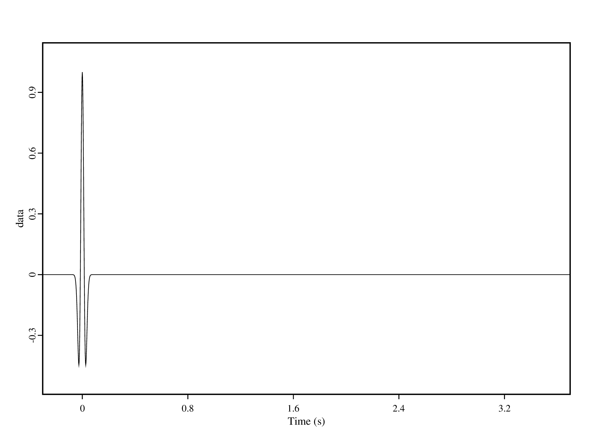
- We create a source of Ricker wavelet with peak frequency 30Hz. The source is planning to be fired at 3000m in lateral position and 10 meter deep in the water.
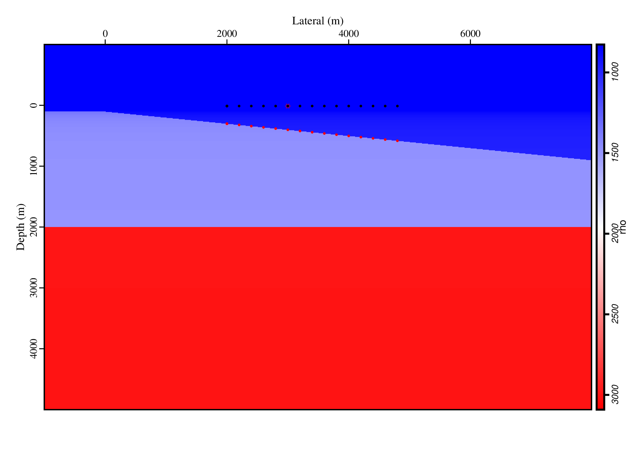
- Now we create two observation geometries: a hydrophone streamer on the water surface, and a geophone array on the water bottom, and store them as two columns in a single dataset data/rr.sg.
- At last, we do the finite difference wavefield modelling. It has three inputs: the source, the velocity model, and the observation geometry. All of them are stored in the same format, supported by the sigclear-soig.
from experiment import *

Process('vel', None,
	'''
	sgcreate data.s0=-1000 data.ds=10 data.ns=600 nx=900
	| sgfieldmath lateral:f="-1000+jx*10"
	  ref1:f="100+(lateral>0)*0.1*lateral"  ref2:f="2000"
	| sgfieldmath rho:F="1.225+998*(atan(data.time/50)/PI+0.5)"
	  data="340+1160*(data.time>=0)"
	| sgfieldmath rho="rho+500*(data.time>=ref1)+1500*(data.time>=ref2)"
	| sgattribute index=lateral
	  dx:f=10 nx:i=900 ox:f=-1000 ny:i=1
	''')
Figure('./vel.png',
	'''
	sgplotps top.label="Lateral (m)" data.image=bwr rho.image=owb
	''')
Process('source',None,
	'''
	sgcreate data.ns=2000 data.ds=0.002 data.s0=-0.3
	| sgfieldmath index.rename=fldr sz:f=10 sx:f="3000"
	  gy:f=0 sy:f=0 data="ricker(30*data.time)"
	''')
Figure('./source.png', 'sggraphps ')
Process('rr', None,
	'''
	sgcreate data.ns=300 data.ds=10 data.s0=2000 nx=2
	| sgfieldmath index.rename=rl
	  gx:F=data.time gz:F="(jx==0)*10+jx*(100+data.time*0.1)"
	| sgwindow remove=data
	''')
Figure('ss', 'source',
	'''
	sgfieldout fields=sz,sx
	| sggraphps yreverse=y x=sx y=sz
	  sz.style="*" sz.color="FF0000"
	  xmin=-1000 xmax=7990 ymin=-1000 ymax=4990
	''')


Figure('rr', 'rr',
	'''
	sgresamp dt=200
	| sgfieldmath color:i="jx"
	| sggraphps yreverse=y x=gx y=gz
	  gz.style=. gz.color=color
	  xmin=-1000 xmax=7990 ymin=-1000 ymax=4990
	''')

Figure('./obs.png', 'vel ss.ps rr.ps',
	'''
	sgplotps --default=rho rho.top.label="Lateral (m)"
	  rho.image=bwr rho.image.bar=right
	| sgoverlayps ${SOURCES[1:]}
	''')
Process('data wfd', 'source vel rr',
	'''
	sgwefd we=awe2 vel=${SOURCES[1]} vel.vp=data
	  out.grid=${SOURCES[2]} out.grid.vects=gz,gx
	  wfd=${TARGETS[1]}
	''')
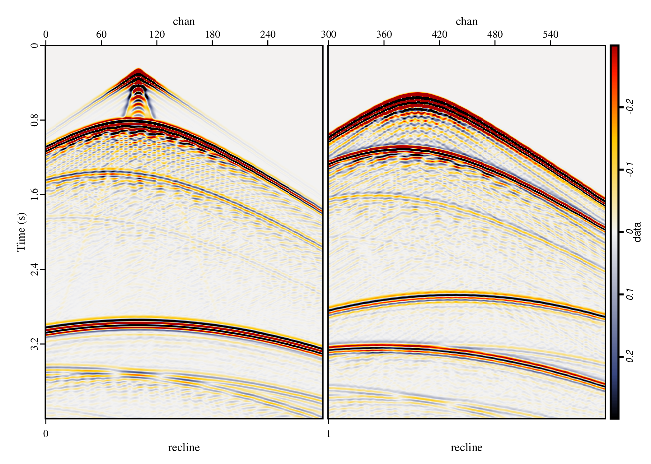
Figure('./data.png',
	'sgplotps data.image=seismic multicol=subgroup')
Figure('./wfd.gif',
	'''
	sgwindow time.min=-0.001 time.max=3.2
	| sgplotps out.title="@group"
	''')