Fit NASA atmospheric pressure measurements.

Overview

From published measurements to a repeatable analysis

This example uses pressure and altitude observations from NASA's Atmospheric Tomography Mission (ATom) Air Age dataset. The workflow imports selected CSV fields, sorts the observations, fits linear and polynomial relationships, and produces comparison figures.

Import measurements

Select the fields needed by the analysis

sgloadcsv reads the pressure and altitude columns. The remaining Programs sort the observations and keep a compact dataset for subsequent Processes.

Process('pressure', './ArN2_AirAge_Trace_Gases.csv',
    '''
    sgloadcsv in.select=pressure,altitude
    | sgsort key=group,altitude
    | sgfieldout fields=pressure,altitude
    ''')

Fit the models

Compare squared-error and robust objectives

The workflow centers altitude before fitting. It then uses sgfit to compare mean squared error (MSE) with mean absolute error (MAE). The same Processes can use a polynomial model by adding model=poly.

Process('fit-linear-mse', 'pressure',
    '''
    sgfieldmath amean:f=altitude.mean altitude=altitude-amean
    | sgfit --default=pressure,altitude
    ''')

Process('fit-linear-mae', 'pressure',
    '''
    sgfieldmath amean:f=altitude.mean altitude=altitude-amean
    | sgfit --default=pressure,altitude norm=mae
    ''')

Because MAE gives extreme residuals less influence than MSE, it provides a useful comparison when measurements contain outliers.

Compare results

Regenerate both comparisons from the same source

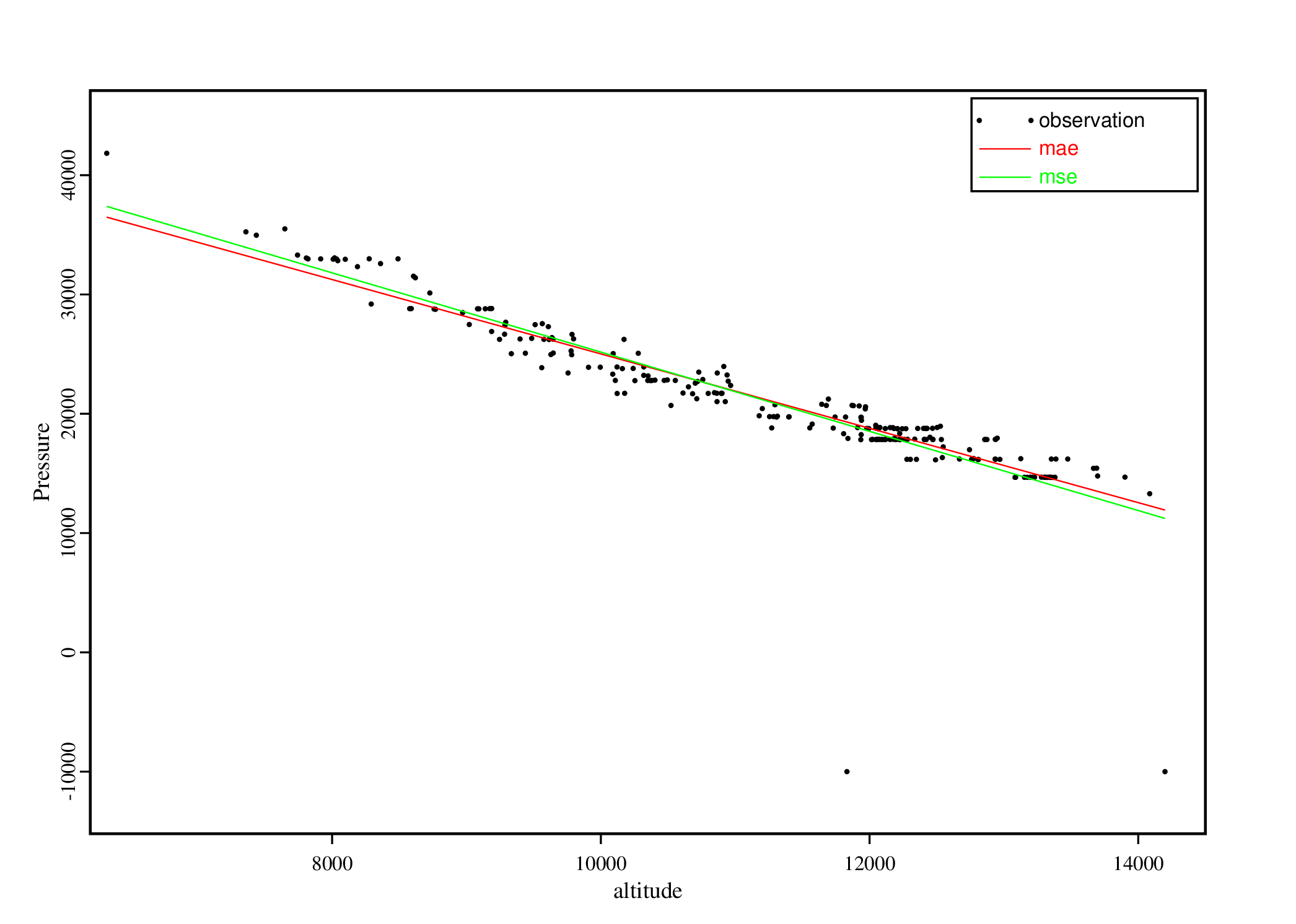Linear models

Compare the sensitivity of MSE and MAE fits to the observations.

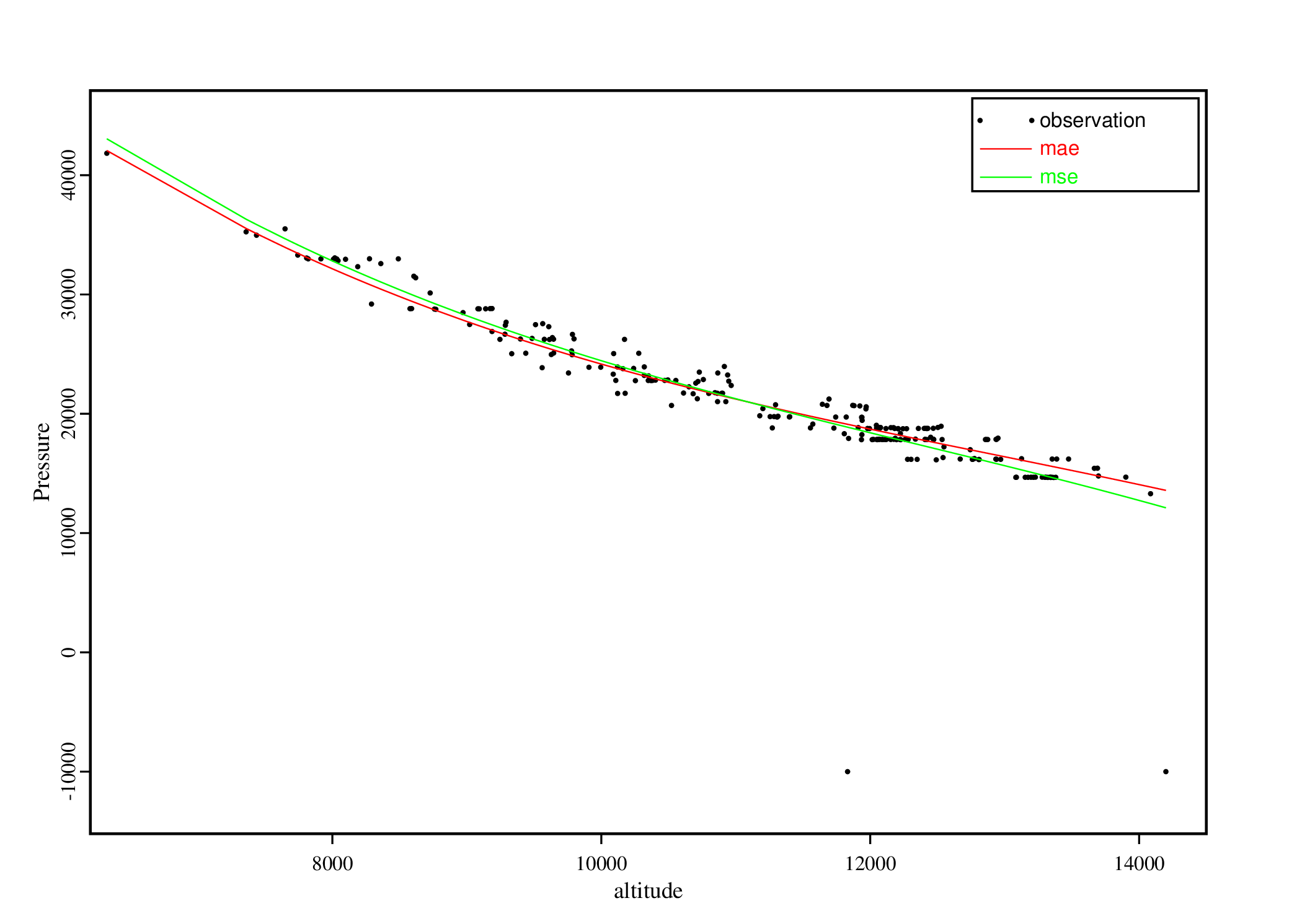Polynomial models

Use the same imported dataset and objectives with a more flexible model.

Resources

Run or adapt the example

The measurements are published as ATom Air Age and trace-gas data, 2009–2018. Download the dataset from its publisher before running the workflow.