Analyze Chang'E-4 lunar radar data.

Overview

Process measurements from the Lunar Penetrating Radar

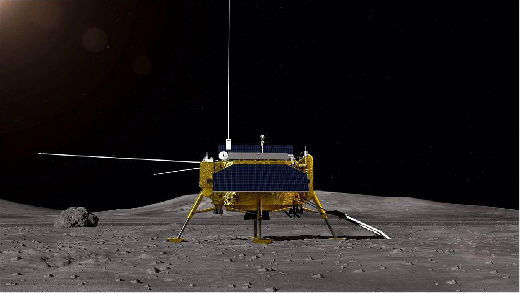
The Chang'E-4 YuTu-2 rover carries a Lunar Penetrating Radar (LPR). This example imports its PDS4 binary records, attaches measurement coordinates and metadata, checks the raw channels, and applies band-pass filtering.

Packages used

sigclear-experiment, sigclear-io, sigclear-soig, sigclear-dsp and sigclear-plot.

Import records

Translate instrument binaries into research datasets

The loading function collects the .2B records for one antenna and passes the binary layout defined by its .2BL description to sgloadbin. It then identifies the dataset keys, calculates acquisition time and sequence fields, and sorts the measurements for downstream processing.

from experiment import *

def LPR_Load(ch, option="", qc=None):
    sources = []
    for item in Glob('DATA/CE4_GRAS_LPR-%s*.2B' % ch):
        sources.append(str(item))

    Process('data-ch%s' % ch, sources,
        '''
        cat ${SOURCES[1:]}
        | sgloadbin %s in.endian=LSB
          out.fields=second,millisec,vel,xpos,ypos,zpos,xref,yref,zref,pitch,roll,yaw,mode,seq_ch1,seq_ch2,antenna,data
          second.format=u32 second.endian=MSB second.start=4
          millisec.format=s16 millisec.endian=MSB
          vel.format=fp32 vel.endian=MSB
          xpos.format=fp32 xpos.endian=MSB
          ypos.format=fp32 ypos.endian=MSB
          zpos.format=fp32 zpos.endian=MSB
          xref.format=fp32 xref.start=38
          yref.format=fp32
          zref.format=fp32
          pitch.format=fp32 pitch.start=50
          roll.format=fp32
          yaw.format=fp32
          mode.format=u8 mode.start=73
          seq_ch1.format=u16 seq_ch1.start=109
          seq_ch2.format=u16
          antenna.format=u8
          data.format=fp32 data.len=2048 data.ds=0.3125
        | sgattribute group:k=second index:k=millisec
        | sgfieldmath time:d="second+0.001*millisec"
          seq:i="(antenna==17)*seq_ch1+(antenna>20)*seq_ch2"
        | sgsort key=xref,seq
        ''' % option)

    if qc is not None:
        Figure('./data-ch%s.png' % ch,
            '''
            sgwindow gmin=%d gmax=%d
            | sgplotps left.label="Time (ns)"
            ''' % (qc, qc))

LPR_Load('1',  "in.colsz=32883 data.len=8192 data.ds=2.5", qc=10)
LPR_Load('2A', "in.colsz=8307 data.len=2048 data.ds=0.3125", qc=10)
LPR_Load('2B', "in.colsz=8307 data.len=2048 data.ds=0.3125", qc=10)

Channel 1 is centered near 60 MHz; channels 2A and 2B are centered near 500 MHz. Their different record and sampling layouts are declared once in the loading function.

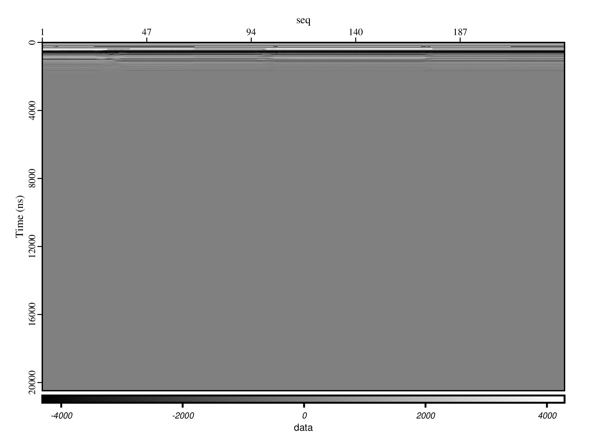
Inspect raw data

Connect quality control to the imported dataset

A specialized Figure Process plots selected radar traces. If the source records or loading parameters change, Workflow Automation regenerates the affected dataset and figure.

Filter channels

Reuse one Process definition across antennas

The filtering function applies zero-phase Butterworth high-pass and low-pass filters. Channel-specific frequency bands are supplied as parameters rather than duplicating the processing and quality-control logic.

from experiment import *

def LPR_FiltBW(ch, fmin=0.04, fmax=0.08, qc=None):
    Process('filtbw-ch%s' % ch, 'data-ch%s' % ch,
        '''
        sgfilterbw phase=zero fc=%f type=highpass
        | sgfilterbw phase=zero fc=%f
        ''' % (fmin, fmax))

    if qc is not None:
        Process('qc-filtbw-ch%s' % ch,
            'data-ch%s filtbw-ch%s' % (ch, ch),
            '''
            sgcat -mode=vector ${SOURCES[1:]}
            | sgwindow gmin=%d gmax=%d
            | sgfieldmath data1.rename=filtbw
            ''' % (qc, qc))

        Figure('./filt-ch%s.png' % ch,
            'qc-filtbw-ch%s' % ch,
            '''
            sggain div.vrms=0.25 div.texp=3
            | sgplotps left.label="Time (ns)"
            ''')

        Figure('./freq-filt-ch%s.png' % ch,
            'qc-filtbw-ch%s' % ch,
            '''
            sgfft1 output=magnitude
            | sgstack
            | sggraphps y=data,filtbw filtbw.color=FF0000
              subtitle="Magnitude (dB)" legend=topright
              bottom.label="Frequency (GHz)"
            ''')

LPR_FiltBW('1',  fmin=0.04, fmax=0.08, qc=0)
LPR_FiltBW('2A', fmin=0.25, fmax=0.75, qc=0)
LPR_FiltBW('2B', fmin=0.25, fmax=0.75, qc=0)

Compare results

Review time- and frequency-domain quality control

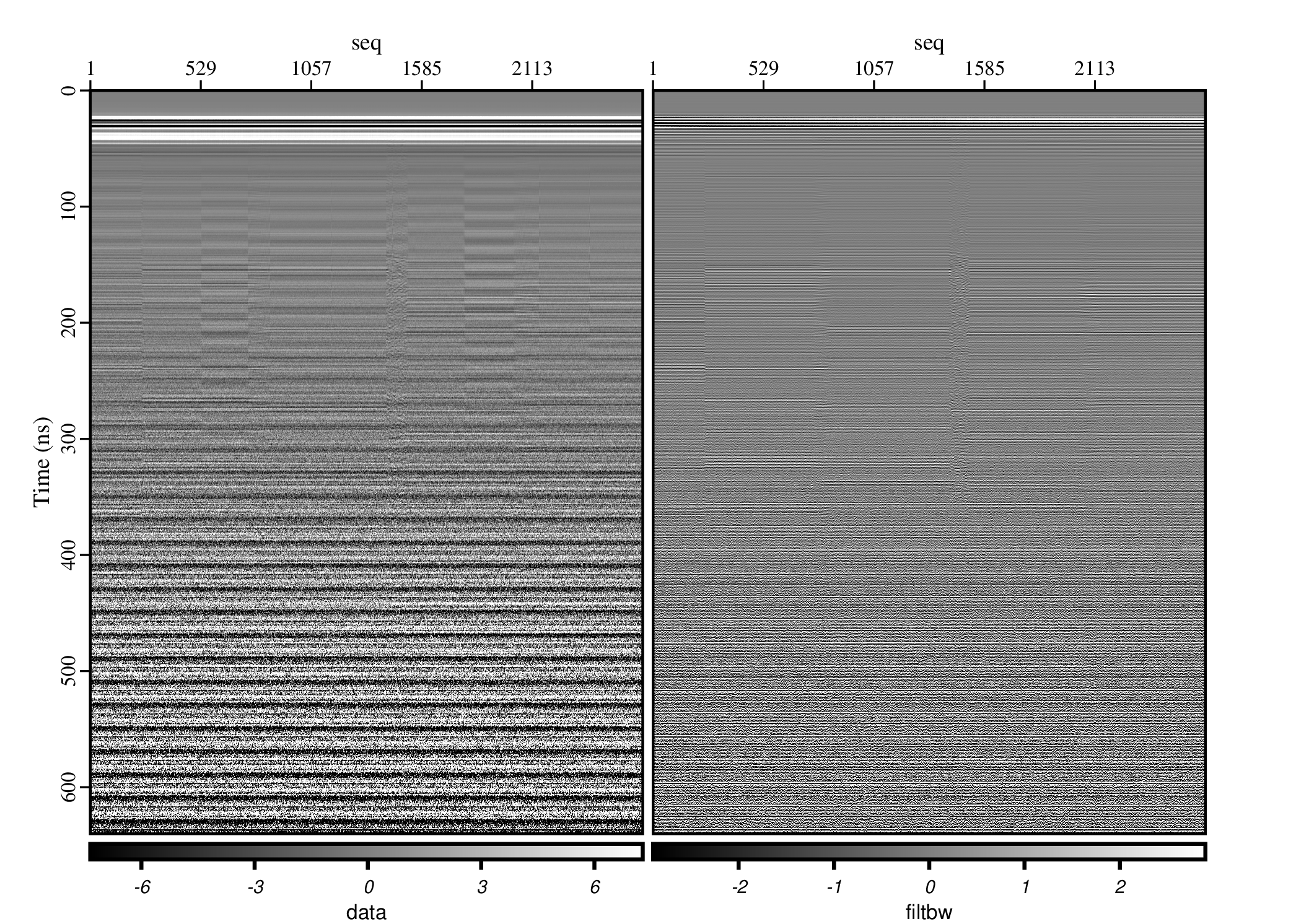Time domain

Compare raw and filtered measurements across radar traces.

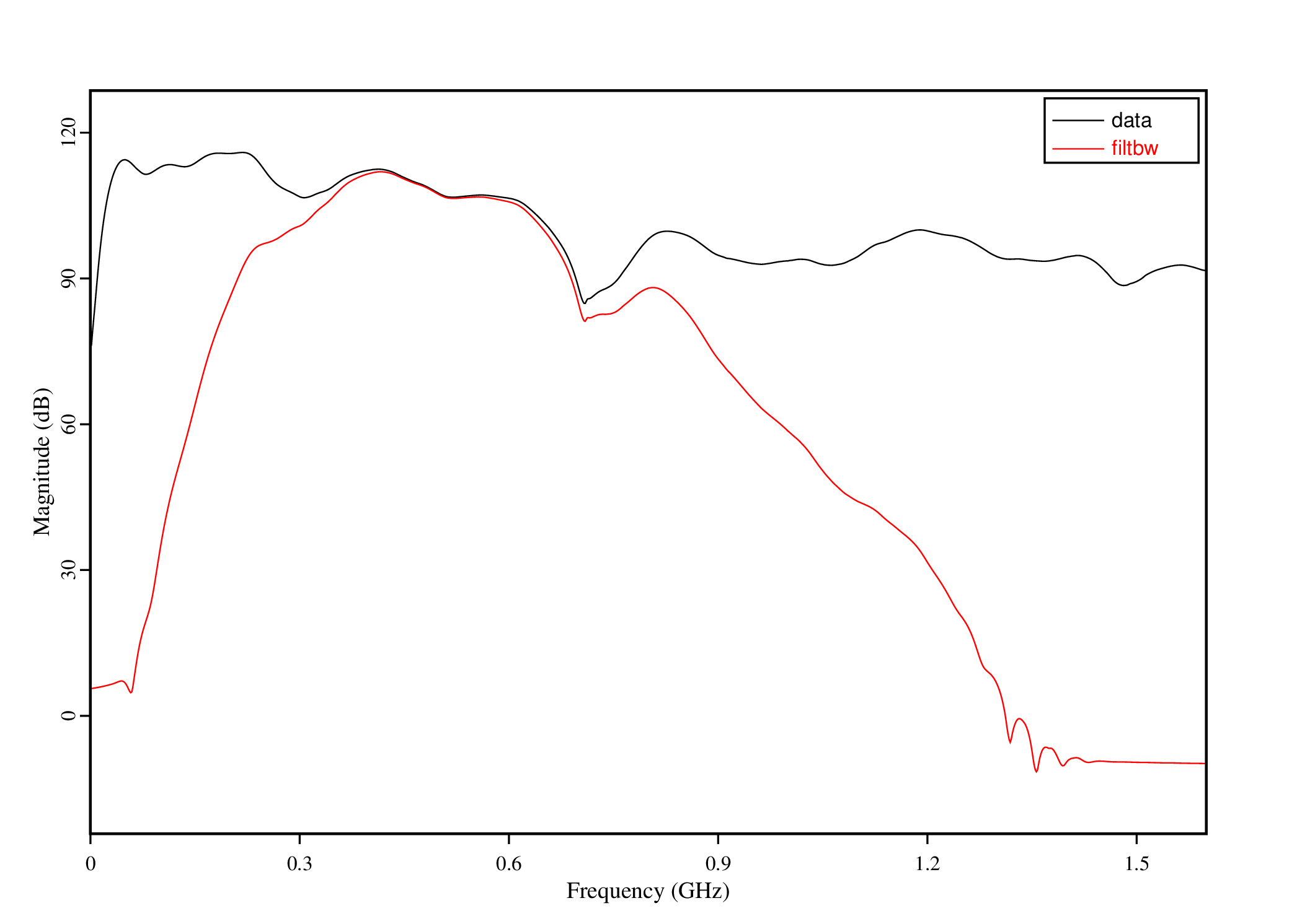Frequency domain

Use Fourier analysis to confirm the effect of the selected pass band.

Resources

Run or adapt the example

Obtain the Chang'E-4 scientific data records from the Lunar and Planetary Data Release System and place the .2B files in a DATA directory beside the downloaded scripts. Run scons from that directory; SConstruct loads both workflow modules.

ce4lpr/
├── SConstruct
├── j01_lpr_load.py
├── j02_lpr_filt.py
└── DATA/
    └── CE4_GRAS_LPR-*.2B

$ cd ce4lpr
$ scons